Computer Graphics 2

Raytracing - Part 1: Setting the Scene

Heather Arbiter — Joe Pietruch

Reverse-engineering a 3D Scene from a 2D image can be a little tricky. Fortunately, I had Heather's help. She had things well underway by the time I met her in the lab, so we tweaked a few parameters and made the render seen below. We used the Bryce 3D editor because it's a quick and easy way to visually set up the scene. The one on the left is what we were attempting to recreate, and on the right is our result.

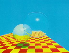
As you can see, it's not quite perfect. The important thing, however, is the refracting sphere has both the floor and the reflective sphere showing through it, and the reflective sphere reflects the floor and casts a shadow. The positions and sizes of our scene components can be found in the tables below.

Our Parameters

Camera
eye-x	54.90
eye-y	56.55
eye-z	-201.46
fov	61.77
lookat-x	89.54
lookat-y	17.10
lookat-z	202.42
near-clip	5
far-clip	500

Floor
x	71.59
y	-20.14
z	96.88
width	197.61
length	401.54

Light
x	71.06
y	162.37
z	-145.73

Sphere (transparent)
x	74.40
y	44.10
z	-78.26
radius	21.86

Sphere (reflective)
x	46.71
y	26.02
z	-32.30
radius	18.90

---

Raytracing - Part 2: Camera Modeling

Joe Pietruch — Heather Arbiter

I have to say, I'm liking C# MUCH better than C++. None of this troubleshooting little intricacies and idiosyncracies of the language. If something goes wrong, I know it's my own fault, and the error messages tell me how to fix it! Thank goodness!

That said, it was a little interesting trying to set up a camera without being able to see it. I'm accustomed to working in a 3D Modelling GUI and being given a visualization of the scene easy. We traced out the numbers, and they seemed correct, so we had no choice but to trust them. When we finally got it going it made us quite happy! The image on the left shows our original results, the right is a supersampled image (click for full size):

---

Raytracing - Part 3: Basic Shading

Joe Pietruch — Heather Arbiter

We added materials to our objects so that they had physical properties which could be used with the Phong lighting. We also updated our code structure to move some segments of code into more logical places.

We ran into some unexpected (though artistically wonderful!) results with the specular calculations. The image below shows a highlight on the wrong side of the sphere! One specular highlight is caused by the dot product between the reflection vector and the view vector being positive, the other when the dot product is negative. Once we realized this, it was a simple matter of excluding the lower highlight for the final submission.

Here are two images of our results. The first shows a single white light in the scene. The second has 3 different color lights in a different place to show multiple light sources. The colors of the spheres in that example were changed to white and off-white to make the colored lights easier to see.

---

Raytracing - Part 4: Procedural Shading

Joe Pietruch — Heather Arbiter

We added a procedural shader to the floor of our scene. This was done by finding the intersection point in the coordinate system of our plane, and then determining what the texture coordinates would be at that coordinate. The texture color then replaces the ambient color in the Phong equation.

Here are two images of our results. The first shows our basic procedural checkerboard pattern. The second is a target-shaped pattern formed by taking the length of the UV coords (treated as a vector) and splitting it up into odd/even circles in the same way the checkers were odd/even squares.

---

Raytracing - Part 5: Recursive Reflection

Joe Pietruch — Heather Arbiter

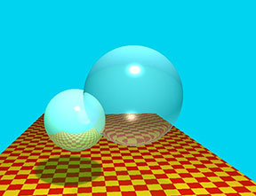
We made our illumination function recursive, which is the easy way to add reflections to a raytraced image. I think it came out very well. We were fortunate to avoid some of the hairy reflection math because the vector library we're using came with a static Reflection() function.

Here are two images of our results. The first shows reflection on one sphere. The second applies the reflection to both spheres, and because our depth is three we get reflections of reflections of reflections. Hooray!

---

Raytracing - Part 6: Recursive Refraction

Joe Pietruch — Heather Arbiter

Not content with bouncing around the outside of our spheres, we ventured into the realm of transmissive rays. As seen below the larger sphere is now partially transparent. I ran into some difficulty programming this one. For a while, my refractions behaved just like reflections, and this discouraged me. With a little help (I find it much easier to debug when I can bounce ideas off of people!) I finally figured out that I was switching parity too often and in the wrong places. In the process of fixing it I got a little overzealous with my wiggle fudge-factor vector, as seen below.

The results were promising. Below on the left is the normal image for this checkpoint. We went a step beyond with the image on the right, our refracted-shadow-ray extra. The strategy invovled refracting the shadow ray through the sphere, and then comparing the emerging ray's normal with the normal pointing at the light. Their dot product determined the relative intensity of transmitted light. I'm not entirely sure why it came out more dense than the regular shadow.

Adding the specular component in had two interesting results. First, it generated a lot of noise on the spheres. I looked as hard as I could for a rounding error, with no luck finding it. Second, it seemed to simulate some caustic effects. Encouraged by this, I supersampled the image, and the noise cleared itself up a bit. I'm beginning to wonder if it's a sampline problem and not roundoff afterall? The "focused" specular highlight, as well as the rimming along the sphere and shadow edge make for a neat effect. With more rays (I only shot four) it might just smooth itself out!

---

Raytracing - Part 7: Tone Reproduction

Joe Pietruch — Heather Arbiter

In our case, tone reproduction is really a post-processing step over all the pixels in the generated image. What you see below is our original rendering (without any tone reproduction) which is the base condition for each of the following images. In the table are our two different models used for tone reproduction (Ward and Reinhard) rendered at different scene luminances. Note that Ward's model is meant to exhibit a perceptual change under different lighting conditions, while Reinhard's model is meant to simulate a camera metering under different lighting conditions (in a perfect world, a camera metering system will produce a consistant exposure across all lighting conditions!).

	Ward	Reinhard
1.0 cd/m^2
1000 cd/m^2
10000 cd/m^2

As an extra bonus, I rendered out Ansel Adams' "Zone System" through Reinhard's tone reproduction. Each successive image is one stop away from the other up the scale.

I	II	III	IV	V	VI	VII	VIII	IX	X